
GPT 4o- with Canvas: Data Analysis has changed once again!
OpenAI has released a new feature!


Three days ago, OpenAI released a new feature of GPT 4o with Canvas. If you are familiar with artifacts in Claude, it is similar.
But, by using this feature, you can ease your Data Analysis. In this article, we’ll explore how you can do it together. To do that, we’ll use the Global Earthquake dataset from Kaggle.
Global Earthquake Data

This dataset has 43 attributes, such as magnitude, location, depth, and seismological measurements, that provide detailed information on 1,137 earthquakes worldwide.
GPT 4o- with Canvas
Now first, let’s select this model from the available model list.

Great. Now, let’s use this prompt structure, which will help you analyze the given dataset wisely. But before that, upload the dataset you downloaded from Kaggle.
Here is the dataset information
[Paste Dataset information from Kaggle]
Write me a machine learning code that predicts magnitude of earthquakes.
Here is the code.
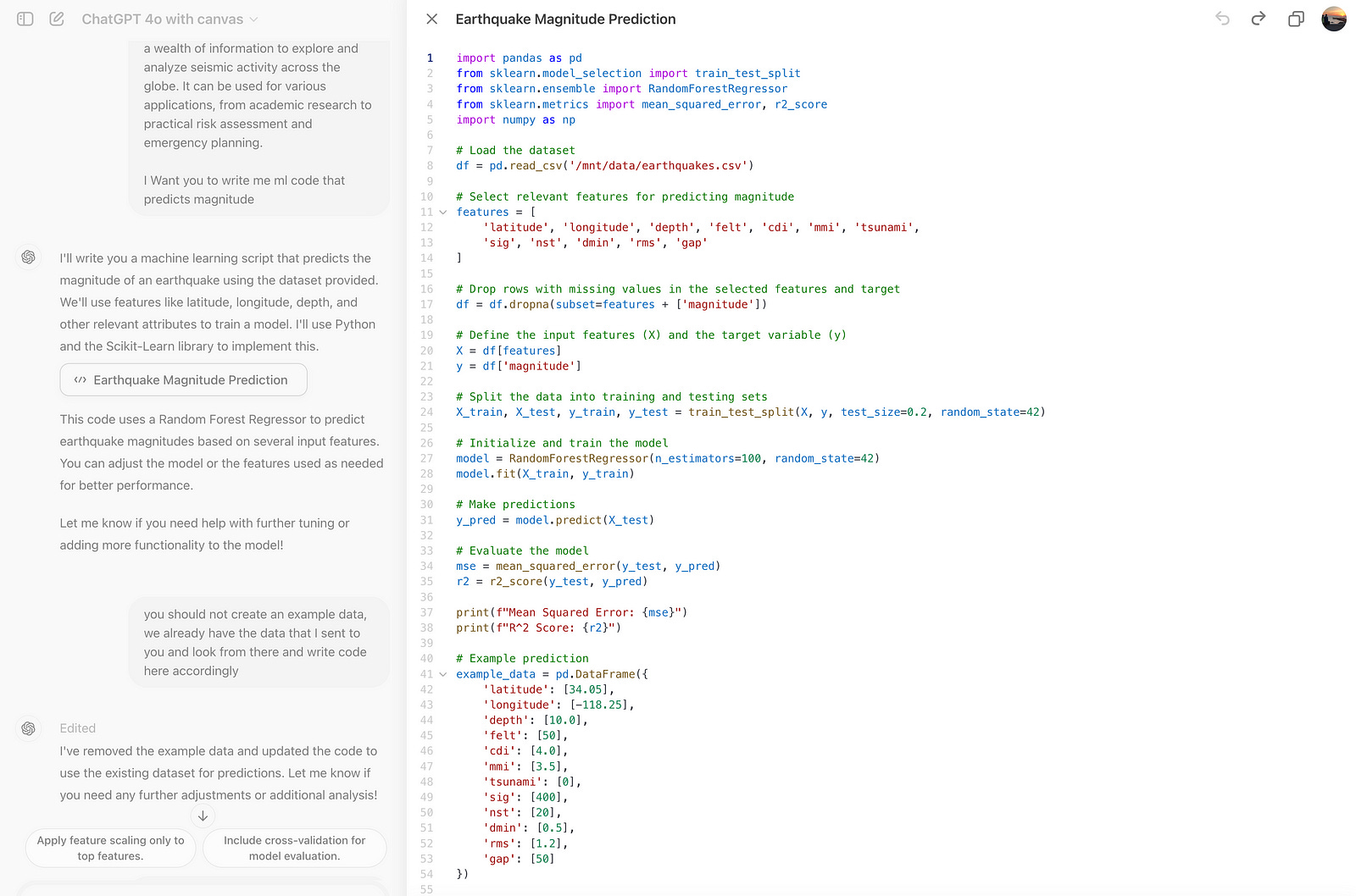
But did you notice that it created its dataset instead of using the one we uploaded? It is okey; LLMs can make mistakes once in a while, and that’s why they still need humans.
Here is the prompt to adjust it.
You should not create an example data, we already have the data that I sent to you an
look from there and write code here accordingly
Here.
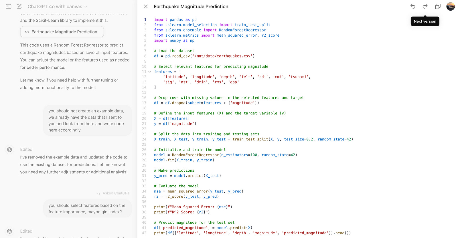
As you can see, it uses our dataset, but this time, it selects features that it writes itself. We need to change that.
Here is the prompt that I’ve used.
you should select features based on the feature importance, maybe gini index?Now, let’s feed information to ChatGPT.
Here all features.
[paste df.info codes output here- all column names]
You should select all at first, and then label encoding then and
select important ones with gini
Here, I’ve realized that we used too many different methods to create the best models like;
Normalization
Apply 5 Different ML models
Select different models with gini importance
Log transformation
Dimension Reduction
I asked Gpt 4o with Canvas to create codes by adding the methods above. Here is my final code.
import pandas as pd
from sklearn.model_selection import train_test_split
from sklearn.ensemble import RandomForestRegressor, GradientBoostingRegressor
from sklearn.linear_model import LinearRegression
from sklearn.tree import DecisionTreeRegressor
from sklearn.svm import SVR
from sklearn.metrics import mean_squared_error, r2_score
from sklearn.preprocessing import LabelEncoder, StandardScaler, MinMaxScaler
from sklearn.decomposition import PCA
import numpy as np
import matplotlib.pyplot as plt
# Load the dataset
df = pd.read_csv('/mnt/data/earthquakes.csv')# Select all features initially
all_features = df.columns.tolist()
all_features.remove('magnitude') # Remove target variable from features# Handle categorical features using Label Encoding
categorical_features = df.select_dtypes(include=['object']).columns
label_encoders = {}
for feature in categorical_features:
le = LabelEncoder()
df[feature] = le.fit_transform(df[feature].astype(str))
label_encoders[feature] = le# Drop rows with missing values in the selected features and target
df = df.dropna(subset=all_features + ['magnitude'])# Define the input features (X) and the target variable (y)
X = df[all_features]
y = df['magnitude']# Check for skewness and apply log transformation where necessary
for col in X.columns:
if X[col].skew() > 1 or X[col].skew() < -1:
X.loc[:, col] = np.log1p(X[col])# Normalize the features using StandardScaler
scaler_standard = StandardScaler()
X_standard = scaler_standard.fit_transform(X)# Normalize the features using MinMaxScaler
scaler_minmax = MinMaxScaler()
X_minmax = scaler_minmax.fit_transform(X)# Dimensionality Reduction using PCA (if number of features is high)
pca_threshold = 0.95
if X_standard.shape[1] > 10:
pca_standard = PCA(n_components=pca_threshold)
X_standard = pca_standard.fit_transform(X_standard)
pca_minmax = PCA(n_components=pca_threshold)
X_minmax = pca_minmax.fit_transform(X_minmax)# Split the data into training and testing sets for both normalization methods
X_train_standard, X_test_standard, y_train, y_test = train_test_split(X_standard, y, test_size=0.2, random_state=42)
X_train_minmax, X_test_minmax, _, _ = train_test_split(X_minmax, y, test_size=0.2, random_state=42)# Initialize RandomForestRegressor to determine feature importance
feature_importance_model = RandomForestRegressor(n_estimators=100, random_state=42)
feature_importance_model.fit(X_train_standard, y_train)# Calculate feature importance using the features used in the training set after transformations
actual_features = X.columns[:X_train_standard.shape[1]]
feature_importances = feature_importance_model.feature_importances_
feature_importance_df = pd.DataFrame({'feature': actual_features, 'importance': feature_importances})
feature_importance_df = feature_importance_df.sort_values(by='importance', ascending=False)# Select the most important features (top 8 and top 10)
top_8_features = feature_importance_df['feature'].head(8).tolist()
top_10_features = feature_importance_df['feature'].head(10).tolist()# Define input features for top 8 and top 10 feature sets
X_top_8 = df[top_8_features].copy()
X_top_10 = df[top_10_features].copy()# Check for skewness in top features and apply log transformation where necessary
for col in X_top_8.columns:
if X_top_8[col].skew() > 1 or X_top_8[col].skew() < -1:
X_top_8.loc[:, col] = np.log1p(X_top_8[col])
for col in X_top_10.columns:
if X_top_10[col].skew() > 1 or X_top_10[col].skew() < -1:
X_top_10.loc[:, col] = np.log1p(X_top_10[col])# Normalize the selected top features using both scalers
X_top_8_standard = scaler_standard.fit_transform(X_top_8)
X_top_8_minmax = scaler_minmax.fit_transform(X_top_8)
X_top_10_standard = scaler_standard.fit_transform(X_top_10)
X_top_10_minmax = scaler_minmax.fit_transform(X_top_10)# Dimensionality Reduction using PCA for top 8 and top 10 features
if X_top_8_standard.shape[1] > 5:
pca_top_8_standard = PCA(n_components=pca_threshold)
X_top_8_standard = pca_top_8_standard.fit_transform(X_top_8_standard)
pca_top_8_minmax = PCA(n_components=pca_threshold)
X_top_8_minmax = pca_top_8_minmax.fit_transform(X_top_8_minmax)
if X_top_10_standard.shape[1] > 5:
pca_top_10_standard = PCA(n_components=pca_threshold)
X_top_10_standard = pca_top_10_standard.fit_transform(X_top_10_standard)
pca_top_10_minmax = PCA(n_components=pca_threshold)
X_top_10_minmax = pca_top_10_minmax.fit_transform(X_top_10_minmax)# Split the data for top 8 and top 10 feature sets
X_train_8_standard, X_test_8_standard, _, _ = train_test_split(X_top_8_standard, y, test_size=0.2, random_state=42)
X_train_8_minmax, X_test_8_minmax, _, _ = train_test_split(X_top_8_minmax, y, test_size=0.2, random_state=42)
X_train_10_standard, X_test_10_standard, _, _ = train_test_split(X_top_10_standard, y, test_size=0.2, random_state=42)
X_train_10_minmax, X_test_10_minmax, _, _ = train_test_split(X_top_10_minmax, y, test_size=0.2, random_state=42)# Define the models to be used
models = {
'Random Forest': RandomForestRegressor(n_estimators=100, random_state=42),
'Gradient Boosting': GradientBoostingRegressor(n_estimators=100, random_state=42),
'Linear Regression': LinearRegression(),
'Decision Tree': DecisionTreeRegressor(random_state=42),
'Support Vector Regressor': SVR()
}# Train each model and evaluate performance for each combination
model_results = {}
normalizations = [
('StandardScaler - Top 8 Features', X_train_8_standard, X_test_8_standard),
('MinMaxScaler - Top 8 Features', X_train_8_minmax, X_test_8_minmax),
('StandardScaler - Top 10 Features', X_train_10_standard, X_test_10_standard),
('MinMaxScaler - Top 10 Features', X_train_10_minmax, X_test_10_minmax)
]for normalization_name, X_train, X_test in normalizations:
for model_name, model in models.items():
model.fit(X_train, y_train)
y_pred = model.predict(X_test)
mse = mean_squared_error(y_test, y_pred)
r2 = r2_score(y_test, y_pred)
model_results[f'{model_name} ({normalization_name})'] = {'MSE': mse, 'R2': r2}
print(f"{model_name} ({normalization_name}) - Mean Squared Error: {mse}, R^2 Score: {r2}")# Plot the results
model_names = list(model_results.keys())
mse_values = [model_results[name]['MSE'] for name in model_names]
r2_values = [model_results[name]['R2'] for name in model_names]fig, ax = plt.subplots(1, 2, figsize=(20, 10))# Bar plot for MSE
ax[0].barh(model_names, mse_values, color='skyblue')
ax[0].set_title('Mean Squared Error Comparison')
ax[0].set_xlabel('MSE')# Bar plot for R2 Score
ax[1].barh(model_names, r2_values, color='lightgreen')
ax[1].set_title('R^2 Score Comparison')
ax[1].set_xlabel('R^2 Score')plt.tight_layout()
plt.show()Here is the output’s first part.
Random Forest (StandardScaler - Top 8 Features) - Mean Squared Error: 0.036684462750000014, R^2 Score: 0.8779777294037107
Gradient Boosting (StandardScaler - Top 8 Features) - Mean Squared Error: 0.03171284438291409, R^2 Score: 0.8945146531096477
Linear Regression (StandardScaler - Top 8 Features) - Mean Squared Error: 0.2030328908150269, R^2 Score: 0.3246586569411304
Decision Tree (StandardScaler - Top 8 Features) - Mean Squared Error: 0.014955, R^2 Score: 0.9502556962820041
Support Vector Regressor (StandardScaler - Top 8 Features) - Mean Squared Error: 0.19093007009631902, R^2 Score: 0.3649158545122343
Random Forest (MinMaxScaler - Top 8 Features) - Mean Squared Error: 0.0368944044999999, R^2 Score: 0.8772794073592385
Gradient Boosting (MinMaxScaler - Top 8 Features) - Mean Squared Error: 0.02585888543990656, R^2 Score: 0.9139864760192863
Linear Regression (MinMaxScaler - Top 8 Features) - Mean Squared Error: 0.2030123102574625, R^2 Score: 0.3247271133440839
Decision Tree (MinMaxScaler - Top 8 Features) - Mean Squared Error: 0.021312499999999988, R^2 Score: 0.9291089620200744
Support Vector Regressor (MinMaxScaler - Top 8 Features) - Mean Squared Error: 0.1900837276420734, R^2 Score: 0.3677310143981205
Random Forest (StandardScaler - Top 10 Features) - Mean Squared Error: 0.014616167999999801, R^2 Score: 0.9513827415456206
Gradient Boosting (StandardScaler - Top 10 Features) - Mean Squared Error: 0.005215391903357051, R^2 Score: 0.9826522207389522
Linear Regression (StandardScaler - Top 10 Features) - Mean Squared Error: 0.024659998640491166, R^2 Score: 0.9179742920723531
Decision Tree (StandardScaler - Top 10 Features) - Mean Squared Error: 0.01719999999999999, R^2 Score: 0.9427882297593093
Support Vector Regressor (StandardScaler - Top 10 Features) - Mean Squared Error: 0.012001988809648145, R^2 Score: 0.9600781961506436
Random Forest (MinMaxScaler - Top 10 Features) - Mean Squared Error: 0.013746897999999952, R^2 Score: 0.9542741645408019
Gradient Boosting (MinMaxScaler - Top 10 Features) - Mean Squared Error: 0.0066618489718651116, R^2 Score: 0.9778409201885739
Linear Regression (MinMaxScaler - Top 10 Features) - Mean Squared Error: 0.024620634208737134, R^2 Score: 0.918105228631956
Decision Tree (MinMaxScaler - Top 10 Features) - Mean Squared Error: 0.02131249999999998, R^2 Score: 0.9291089620200744
Support Vector Regressor (MinMaxScaler - Top 10 Features) - Mean Squared Error: 0.01063026736761726, R^2 Score: 0.9646409061492308
Here is the graph.
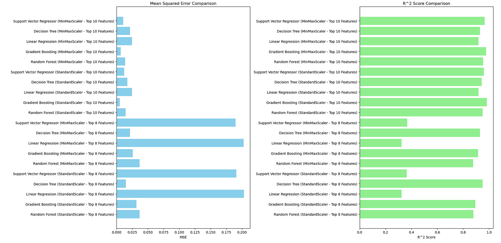
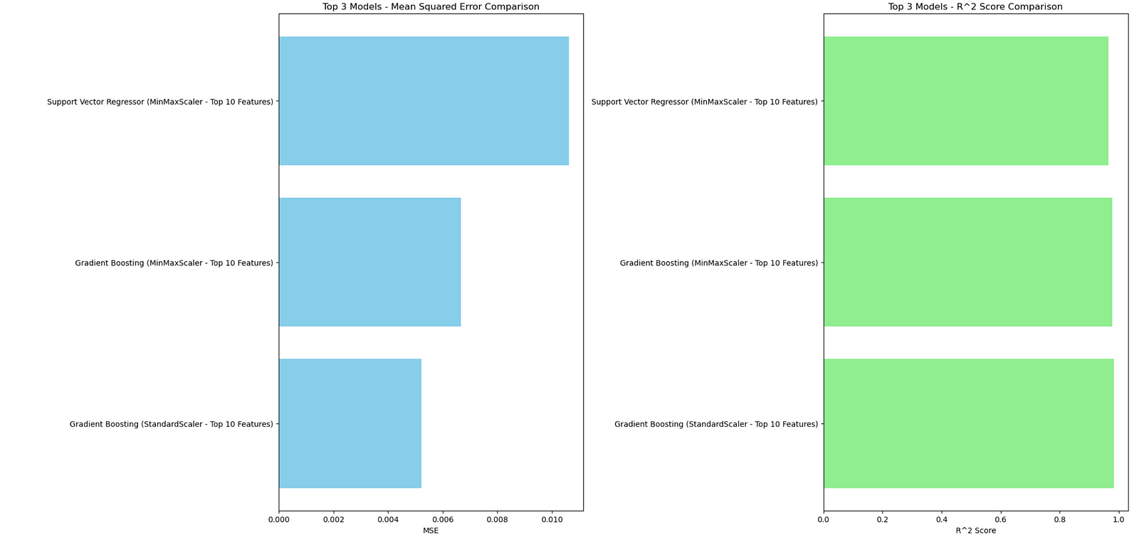
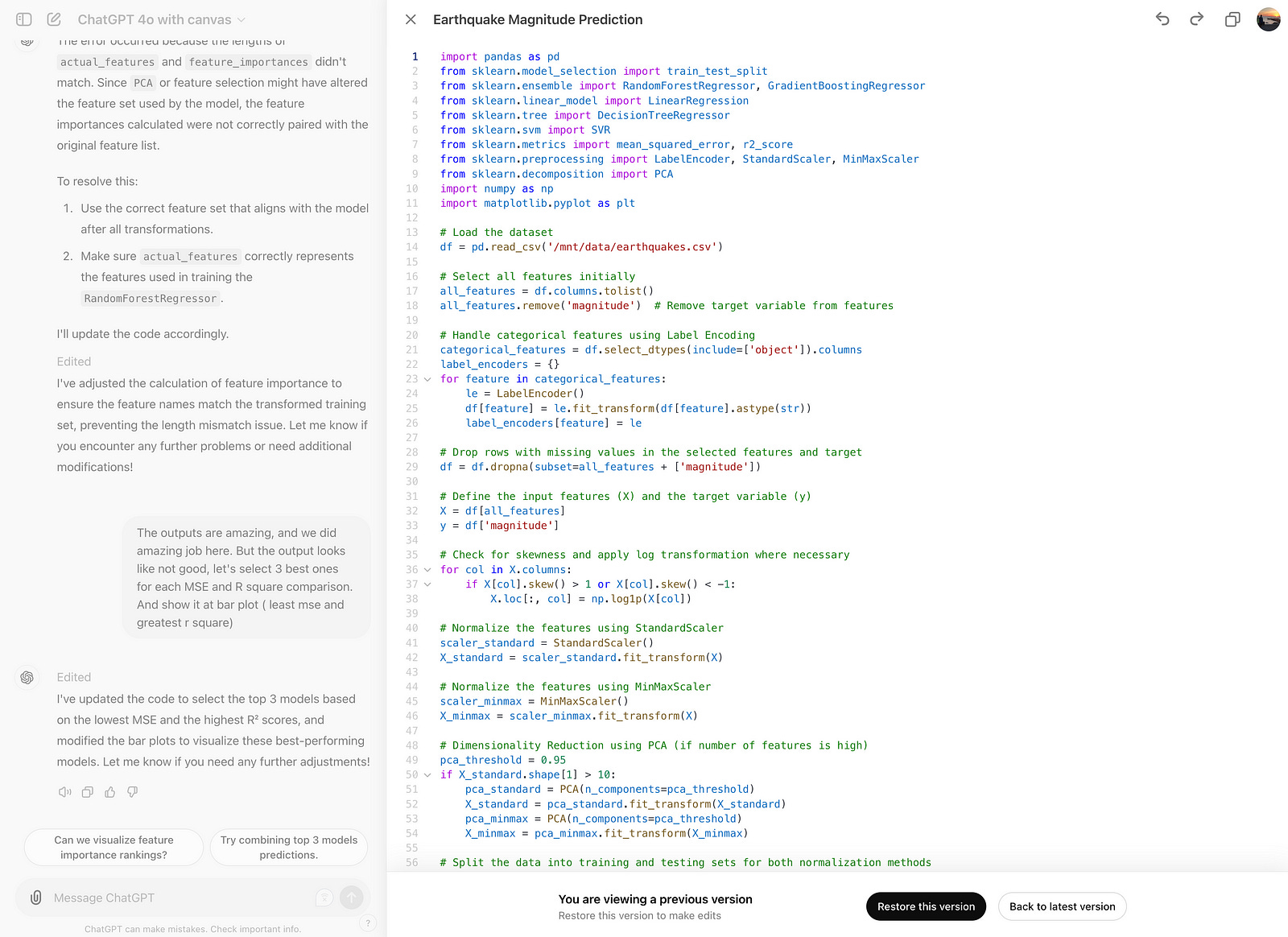
The outputs are unique, and we did a fantastic job here. But the output looks bad. Select the best ones for each MSE and R square comparison.
I pasted the above paragraph to the Gpt 4o-canvas, and it gave me the code. Here is the result.
Versions
Now, if you click on the arrow at the top right, you will see the previous versions of the codes. So, you can also look at the code you have edited.
Check below.
You can also restore this version too.
If you want to automate the data analysis process entirely, use Randy, available for LearnAIWithMe’s paid substack subscribers, from here.

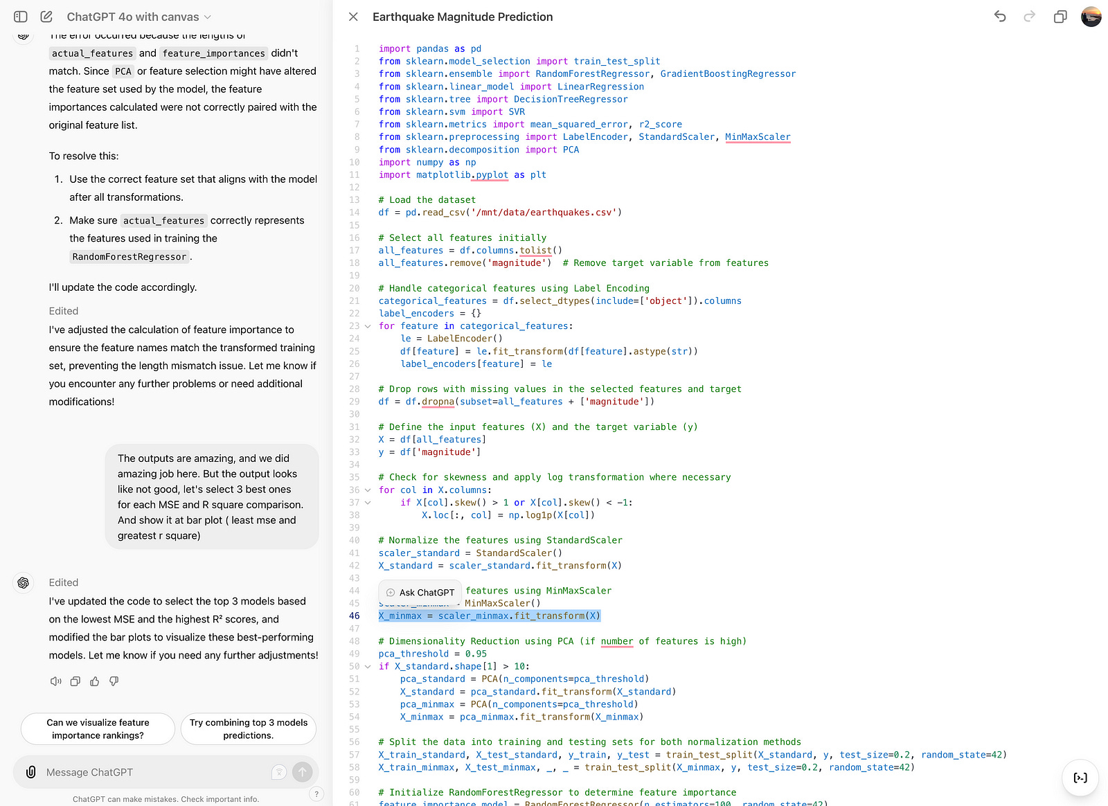
Ask GPT
You can ask GPT to edit this feature by using this feature. Check line 46 below.
Port Language
You can port language, by the way; check it below.
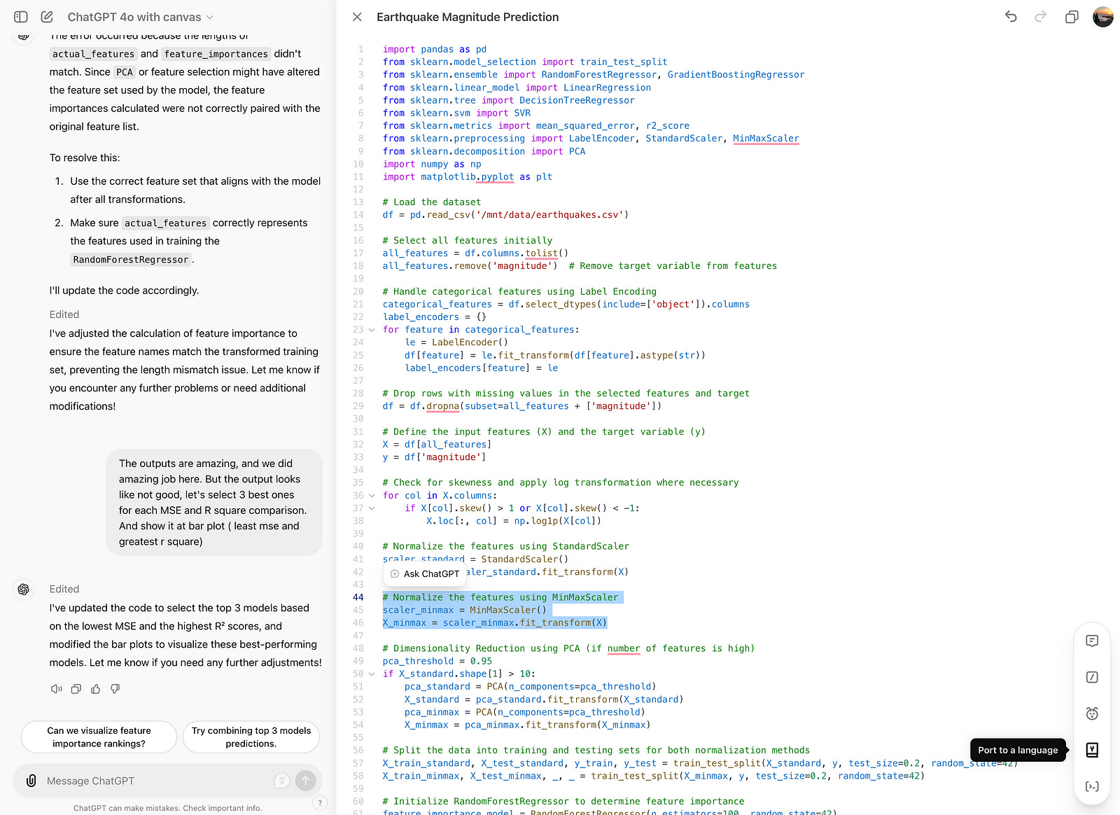
And let’s see how it works. After clicking on it, you will see these options.
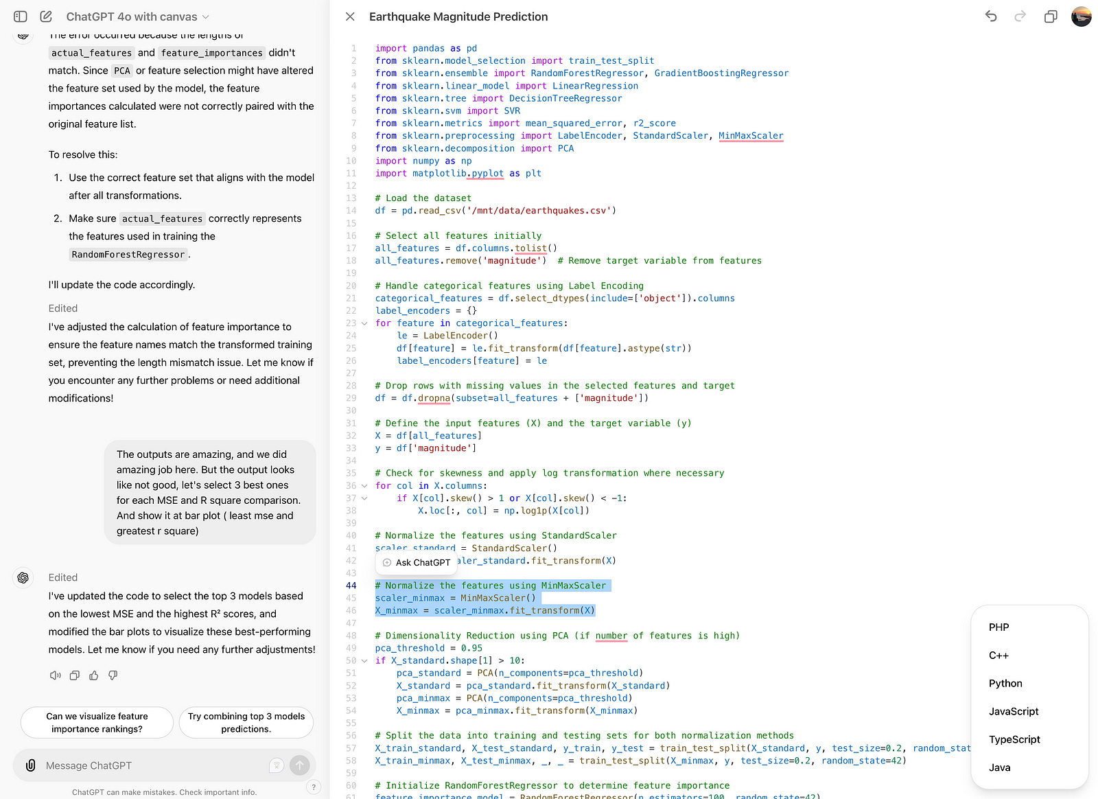
Now I’ve selected Java; here is the result: it has changed the language.
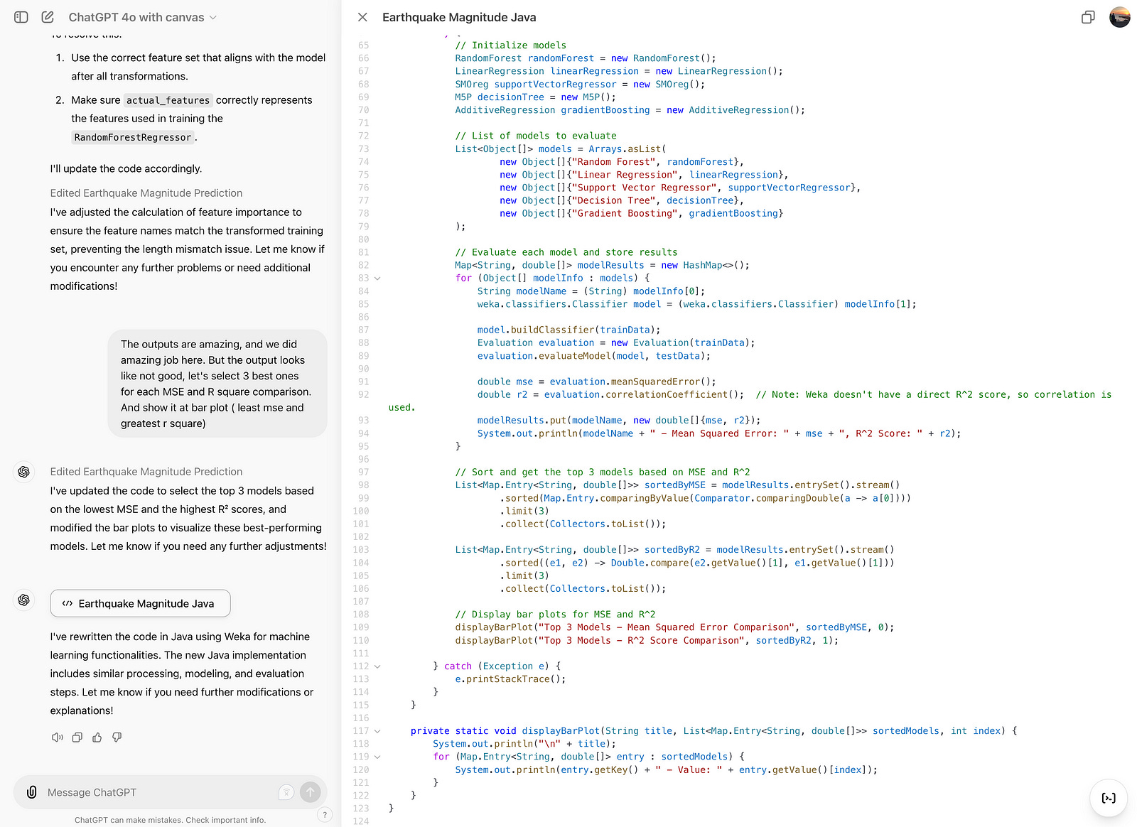
Fix Bugs
Let’s check this feature and fix bugs.
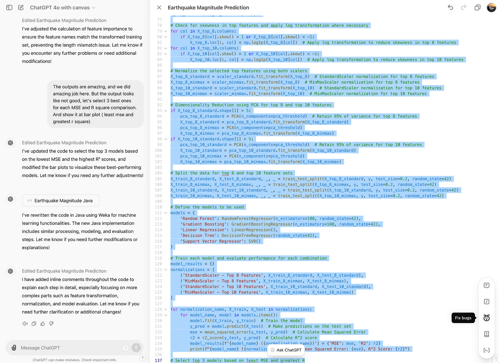
Excellent, it has changed some of the codes.
Add logs
After doing this one, here is the code that it edits.
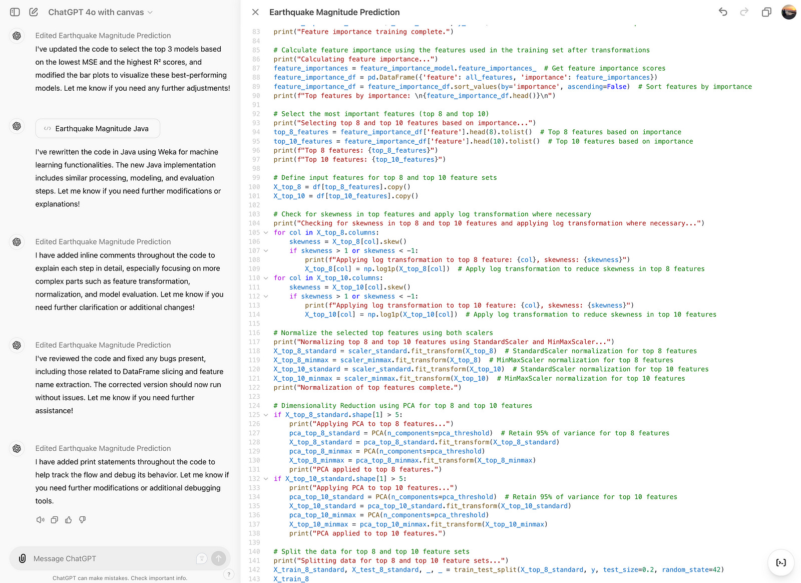
Here is the output.
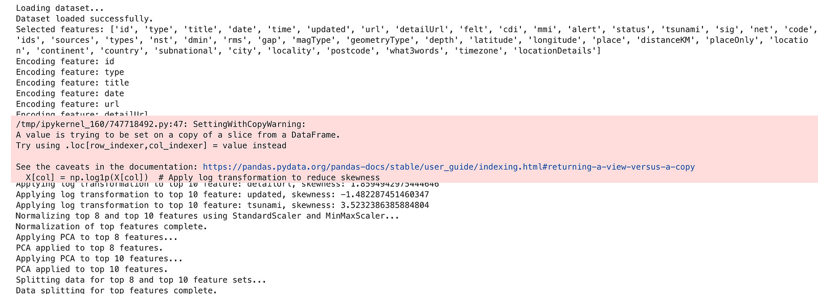
It adds logs to the code, which makes debugging so easier.
Final Thoughts
This article has discovered different GPT 4o-canvas features using a dataset from Kaggle. There is a lot to learn, especially by using new features.
“Machine learning is the last invention that humanity will ever need to make.”
Nick Bostrom